Running a Simulation with metaRVM
Source:vignettes/running-a-simulation.Rmd
running-a-simulation.RmdIntroduction
This vignette demonstrates how to run a metaRVM
simulation using the example configuration and data files included with
the package. This is a good way to get started and understand the basic
workflow.
Locating the Example Files
The metaRVM package includes a set of example files in
its extdata directory. To run the example, these files must
first be located. The system.file() function in R is the
recommended way to do this, as it finds the files wherever the package
is installed.
# Locate the example YAML configuration file
yaml_file <- system.file("extdata", "example_config.yaml", package = "MetaRVM")
print(yaml_file)
#> [1] "/home/runner/work/_temp/Library/MetaRVM/extdata/example_config.yaml"
The yaml_file variable now holds the full path to the
example configuration file. This file is set up to use the other example
data files (also in the extdata directory) with relative
paths. Below is the content of the yaml file.
run_id: ExampleRun
population_data:
  initialization: population_init_n24.csv
  vaccination: vaccination_n24.csv
mixing_matrix:
  weekday_day: m_weekday_day.csv
  weekday_night: m_weekday_night.csv
  weekend_day: m_weekend_day.csv
  weekend_night: m_weekend_night.csv
disease_params:
  ts: 0.5
  ve: 0.4
  dv: 180
  dp: 1
  de: 3
  da: 5
  ds: 6
  dh: 8
  dr: 180
  pea: 0.3
  psr: 0.95
  phr: 0.97
simulation_config:
  start_date: 01/01/2023 # m/d/Y
  length: 150
  nsim: 1
  nrep: 1
  simulation_mode: deterministic
  random_seed: 42
Running the Simulation
Once the path to the configuration file is available, the simulation
can be run using the metaRVM() function.
# Load the metaRVM library
library(MetaRVM)
options(odin.verbose = FALSE)

# Run the simulation
sim_out <- metaRVM(yaml_file)
#> Loading required namespace: pkgbuild
The metaRVM() function will parse the YAML file, read
the associated data files, run the simulation, and return a
MetaRVMResults object.
Deep-dive into MetaRVM Classes
Working with Configuration Files
The simulation can be run by directly providing a YAML configuration
file path, or by creating a MetaRVMConfig object.
# Load configuration from YAML file
config_obj <- MetaRVMConfig$new(yaml_file)

# Examine the configuration
config_obj
#> MetaRVM Configuration Object
#> ============================
#> Config file: /home/runner/work/_temp/Library/MetaRVM/extdata/example_config.yaml
#> Parameters: 42
#> Parameter names (first 10): N_pop, pop_map, category_names, S_ini, E_ini, I_asymp_ini, I_presymp_ini, I_symp_ini, H_ini, D_ini ...
#> Population groups: 24
#> Start date: 2023-09-30
#> Population mapping: [ 24 rows x 4 columns]
Exploring Configuration Parameters
The MetaRVMConfig class provides several methods to
explore the simulation arguments:
# List all available parameters
param_names <- config_obj$list_parameters()
head(param_names, 10)
#>  [1] "N_pop"          "pop_map"        "category_names" "S_ini"
#>  [5] "E_ini"          "I_asymp_ini"    "I_presymp_ini"  "I_symp_ini"
#>  [9] "H_ini"          "D_ini"

# Get a summary of parameter types and sizes
param_summary <- config_obj$parameter_summary()
head(param_summary, 10)
#>                     parameter       type length size
#> N_pop                   N_pop    integer      1    1
#> pop_map               pop_map data.table      4    4
#> category_names category_names  character      3    3
#> S_ini                   S_ini    integer     24   24
#> E_ini                   E_ini    numeric     24   24
#> I_asymp_ini       I_asymp_ini    numeric     24   24
#> I_presymp_ini   I_presymp_ini    numeric     24   24
#> I_symp_ini         I_symp_ini    integer     24   24
#> H_ini                   H_ini    numeric     24   24
#> D_ini                   D_ini    numeric     24   24
Accessing Demographic Information
One of MetaRVM’s key features is demographic stratification, and it’s ability to define parameters for specific demographic strata.
# Get user-defined demographic category names and values
category_names <- config_obj$get_category_names()
cat("Available categories:", paste(category_names, collapse = ", "), "\n")
#> Available categories: age, race, zone

# Example: inspect values for one category (if present)
if ("age" %in% category_names) {
  age_categories <- config_obj$get_category_values("age")
  cat("Age categories:", paste(age_categories, collapse = ", "), "\n")
}
#> Age categories: 0-17, 18-64, 65+
Alternative Ways to Run the Simulation
# Method 1: Direct from file path
# sim_out <- metaRVM(config_file)

# Method 2: From MetaRVMConfig object
sim_out <- metaRVM(config_obj)

# Method 3: From parsed configuration list
config_list <- parse_config(yaml_file)
sim_out <- metaRVM(config_list)
Exploring the Results
The metaRVM() function returns a
MetaRVMResults object with formatted, analysis-ready data.
The results are formatted with calendar dates and demographic
attributes, and stored in a data frame called results:
# Look at the structure of formatted results
head(sim_out$results)
#>          date    age   race  zone disease_state        value instance
#>        <Date> <char> <char> <int>        <char>        <num>    <int>
#> 1: 2023-10-01   0-17      A    11             D 2.252583e-04        1
#> 2: 2023-10-01   0-17      A    11             E 1.365434e+01        1
#> 3: 2023-10-01   0-17      A    11             H 2.304447e-01        1
#> 4: 2023-10-01   0-17      A    11         I_all 2.742619e+01        1
#> 5: 2023-10-01   0-17      A    11       I_asymp 3.555784e-01        1
#> 6: 2023-10-01   0-17      A    11         I_eff 2.483657e+01        1

# Check unique values for key variables
cat("Disease states:", paste(unique(sim_out$results$disease_state), collapse = ", "), "\n")
#> Disease states: D, E, H, I_all, I_asymp, I_eff, I_presymp, I_symp, P, R, S, S_alloc, S_eff_prod, S_src_int, V, V_alloc, V_src_int, cum_V, mob_pop, n_EI, n_EIpresymp, n_HD, n_HR, n_HRD, n_IasympR, n_IsympH, n_IsympR, n_IsympRH, n_RS, n_SE, n_SE_eff, n_SV, n_VE, n_VS, n_preIsymp, p_HRD, p_RS, p_SE, p_VE
cat("Date range:", paste(range(sim_out$results$date), collapse = " to "), "\n")
#> Date range: 2023-10-01 to 2024-02-27
Data Subsetting and Filtering
The subset_data() method provides flexible filtering
across all demographic and temporal dimensions. It returns an object of
class MetaRVMResults.
# Subset by single criteria
hospitalized_data <- sim_out$subset_data(disease_states = "H")
hospitalized_data$results
#>             date    age   race  zone disease_state      value instance
#>           <Date> <char> <char> <int>        <char>      <num>    <int>
#>    1: 2023-10-01   0-17      A    11             H  0.2304447        1
#>    2: 2023-10-01   0-17      A    22             H  0.2081436        1
#>    3: 2023-10-01   0-17      B    11             H  0.5203590        1
#>    4: 2023-10-01   0-17      B    22             H  0.3939861        1
#>    5: 2023-10-01   0-17      C    11             H  0.6244308        1
#>   ---
#> 3596: 2024-02-27    65+      B    22             H  1.2118718        1
#> 3597: 2024-02-27    65+      C    11             H  1.8624622        1
#> 3598: 2024-02-27    65+      C    22             H 10.2755842        1
#> 3599: 2024-02-27    65+      D    11             H  5.5349332        1
#> 3600: 2024-02-27    65+      D    22             H 12.4195984        1

# Subset by multiple demographic categories
elderly_data <- sim_out$subset_data(
  age = c("65+"),
  disease_states = c("H", "D")
)
elderly_data$results
#>             date    age   race  zone disease_state        value instance
#>           <Date> <char> <char> <int>        <char>        <num>    <int>
#>    1: 2023-10-01    65+      A    11             D 2.179919e-05        1
#>    2: 2023-10-01    65+      A    11             H 2.230110e-02        1
#>    3: 2023-10-01    65+      A    22             D 1.453279e-05        1
#>    4: 2023-10-01    65+      A    22             H 1.486740e-02        1
#>    5: 2023-10-01    65+      B    11             D 8.719675e-05        1
#>   ---
#> 2396: 2024-02-27    65+      C    22             H 1.027558e+01        1
#> 2397: 2024-02-27    65+      D    11             D 3.831713e+01        1
#> 2398: 2024-02-27    65+      D    11             H 5.534933e+00        1
#> 2399: 2024-02-27    65+      D    22             D 8.635266e+01        1
#> 2400: 2024-02-27    65+      D    22             H 1.241960e+01        1

# Specific date range
peak_period <- sim_out$subset_data(
  date_range = c(as.Date("2023-10-01"), as.Date("2023-12-31")),
  disease_states = "H"
)
peak_period$results
#>             date    age   race  zone disease_state      value instance
#>           <Date> <char> <char> <int>        <char>      <num>    <int>
#>    1: 2023-10-01   0-17      A    11             H  0.2304447        1
#>    2: 2023-10-01   0-17      A    22             H  0.2081436        1
#>    3: 2023-10-01   0-17      B    11             H  0.5203590        1
#>    4: 2023-10-01   0-17      B    22             H  0.3939861        1
#>    5: 2023-10-01   0-17      C    11             H  0.6244308        1
#>   ---
#> 2204: 2023-12-31    65+      B    22             H  7.0258803        1
#> 2205: 2023-12-31    65+      C    11             H  9.7905521        1
#> 2206: 2023-12-31    65+      C    22             H 52.9246952        1
#> 2207: 2023-12-31    65+      D    11             H 28.3456494        1
#> 2208: 2023-12-31    65+      D    22             H 63.2860726        1
Specifying Disease Parameters via Distributions
metaRVM allows for disease parameters to be specified as
distributions, which is useful for capturing uncertainty. When a
parameter is defined by a distribution, each simulation instance will
draw a new value from that distribution. For more details on the
available distributions and their parameters, refer to the
yaml-configuration vignette.
An example YAML file with parameter distributions is included in the
package, example_config_dist.yaml. Here is its content:
# Locate the example YAML configuration file with distributions
yaml_file_dist <- system.file("extdata", "example_config_dist.yaml", package = "MetaRVM")run_id: ExampleRun_Dist
population_data:
initialization: population_init_n24.csv
vaccination: vaccination_n24.csv
mixing_matrix:
weekday_day: m_weekday_day.csv
weekday_night: m_weekday_night.csv
weekend_day: m_weekend_day.csv
weekend_night: m_weekend_night.csv
disease_params:
ts: 0.5
ve:
dist: uniform
min: 0.3
max: 0.5
dv: 180
dp: 1
de: 3
da:
dist: uniform
min: 4
max: 6
ds:
dist: uniform
min: 5
max: 7
dh:
dist: lognormal
mu: 2
sd: 0.5
dr: 180
pea: 0.3
psr: 0.95
phr: 0.97
simulation_config:
start_date: 01/01/2023 # m/d/Y
length: 150
nsim: 20 # Increased nsim for meaningful summary statistics
nrep: 1
simulation_mode: deterministic
random_seed: 42To run a simulation with this configuration, the file path is passed
to metaRVM.
# Run the simulation with the new configuration
sim_out_dist <- metaRVM(yaml_file_dist)
Generating Summary Statistics across Demographics
The MetaRVMResults class provides basic summarization
functionality across multiple instances of the simulation, when one or
more disease parameters are specified via distribution, and there are
more than one simulations per configurations. The summarize
method generates output of class MetaRVMSummary which has a
plot method available. After a simulation is run with
parameter distributions, the summarize method can be used
to inspect variability in the results.
library(ggplot2)

# Summarize hospitalizations by age group
hospital_summary_dist <- sim_out_dist$summarize(
  group_by = c("age"),
  disease_states = "n_IsympH",
  stats = c("median", "quantile"),
  quantiles = c(0.05, 0.95)
)

# Plot the summary
hospital_summary_dist$plot() + ggtitle("Daily Hospitalizations by Age Group (with 90% confidence interval)") + theme_bw()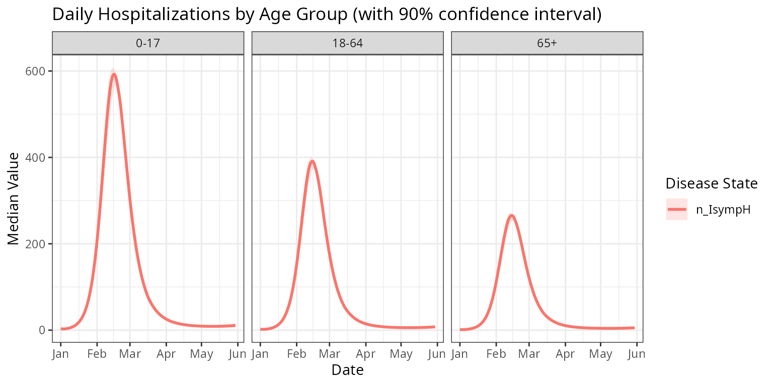
Running a Stochastic Simulation with Static Parameters
A stochastic simulation can also be run by setting
simulation_mode: stochastic.
An example YAML file with parameter distributions is included in the
package, example_config_stochastic.yaml. Here is its
content:
# Locate the example YAML configuration file with distributions
yaml_file_stoch <- system.file("extdata", "example_config_stochastic.yaml", package = "MetaRVM")run_id: ExampleRun_Stochastic_Static
population_data:
initialization: population_init_n24.csv
vaccination: vaccination_n24.csv
mixing_matrix:
weekday_day: m_weekday_day.csv
weekday_night: m_weekday_night.csv
weekend_day: m_weekend_day.csv
weekend_night: m_weekend_night.csv
disease_params:
ts: 0.5
ve: 0.4
dv: 180
dp: 1
de: 3
da: 5
ds: 6
dh: 8
dr: 180
pea: 0.3
psr: 0.95
phr: 0.97
simulation_config:
start_date: 01/01/2023 # m/d/Y
length: 150
nsim: 1
nrep: 5
simulation_mode: stochastic
random_seed: 42
sim_out_stoch <- metaRVM(yaml_file_stoch)Specifying Disease Parameters by Demographics
The disease parameters can also be specified for different
demographic subgroups. These subgroup-specific parameters will override
the global parameters. For more details, refer to the
yaml-configuration vignette. An example YAML file is
provided, example_config_subgroup_dist.yaml, that
demonstrates this feature. It also includes parameters defined by
distributions.
# Locate the example YAML configuration file with subgroup parameters
yaml_file_subgroup <- system.file("extdata", "example_config_subgroup_dist.yaml", package = "MetaRVM")run_id: ExampleRun_Subgroup_Dist
population_data:
initialization: population_init_n24.csv
vaccination: vaccination_n24.csv
mixing_matrix:
weekday_day: m_weekday_day.csv
weekday_night: m_weekday_night.csv
weekend_day: m_weekend_day.csv
weekend_night: m_weekend_night.csv
disease_params:
ts: 0.5
ve:
dist: uniform
min: 0.3
max: 0.5
dv: 180
dp: 1
de: 3
da: 5
ds: 6
dh:
dist: lognormal
mu: 2
sd: 0.5
dr: 180
pea: 0.3
psr: 0.95
phr: 0.97
sub_disease_params:
age:
0-17:
pea: 0.08
18-64:
ts: 0.6
65+:
# This fixed value will override the global lognormal distribution for dh
dh: 10
phr: 0.9227
simulation_config:
start_date: 01/01/2023 # m/d/Y
length: 150
nsim: 20
nrep: 1
simulation_mode: deterministic
random_seed: 42Now, let’s run the simulation with this configuration.
# Run the simulation with the subgroup configuration
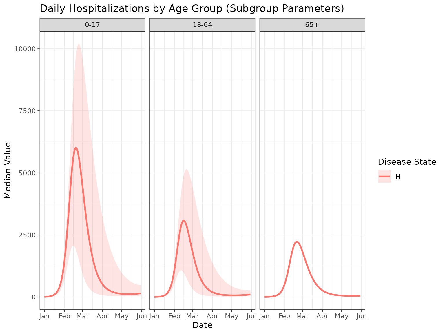
sim_out_subgroup <- metaRVM(yaml_file_subgroup)The results can now be plotted to evaluate the impact of
subgroup-specific parameters. For example, the number of
hospitalizations in the “65+” age group, which has a dh of
10, can be compared to other age groups that use the global
dh drawn from a lognormal distribution.
# Summarize hospitalizations by age group
hospital_summary_subgroup <- sim_out_subgroup$summarize(
  group_by = c("age"),
  disease_states = "H",
  stats = c("median", "quantile"),
  quantiles = c(0.025, 0.975)
)

# Plot the summary
hospital_summary_subgroup$plot() + ggtitle("Daily Hospitalizations by Age Group (Subgroup Parameters)") + theme_bw()